Plot processes

The WPS flyingpigeon provides several processes to perform plot subsetts of netCDF files.

They are several processes to perfom timeseries graphics as well as spatial visualisations as maps.

# birdy client for communication with the server:
from birdy import WPSClient
from os import environ

# handling files and folders
from os import path, listdir
from urllib import request

# wait until WPS process is finished
import time

# to display external png graphics in notebook:
from IPython.display import Image
from IPython.core.display import HTML

# This cell is for server admnistration test purpose
# Ignore this cell and modify the following cell according to your needs

fp_server = environ.get('FYINGPIGEON_WPS_URL')
print(fp_server)  # link to the flyingpigoen server

http://localhost:8093/wps

# URL to a flyingpigeon server
# fp_server = 'https://pavics.ouranos.ca/twitcher/ows/proxy/flyginpigeon/wps'

fp_i = WPSClient(fp_server, progress=True)
fp = WPSClient(fp_server)

read in the required files:

this is an example of an local installation, where local files are processed

indices were calculated with the birdhouse WPS finch: https://finch.readthedocs.io/en/latest/processes.html

# read in the existing indices based on bias_adjusted tas files:
tas_NER = '/home/nils/data/example_data/NER/'
tasInd_NER = [ tas_NER+f for f in listdir(tas_NER) if '.nc' in f ]

tasInd_NER.sort()

pip install pymetalink

# frequencies
freq=['yr','mon']

# precipitation indices
# pr_indices = ['prcptot','rx1day','wetdays','cdd','cwd','sdii','rx5day']
tas_indice = 'tg_mean'

# titles = ['Somme annuelle des précipitations',
#           'Jours de plus fortes précipitations',
#           'Nombre de jours humide',
#           'Journées consécutives de sécheresse',
#           'Jours humides consécutifs',
#           "Index d'intensité de précipitations",
#           'Somme max. sur 5 jours consécutifs',
#           'Températures moyennes annuelles']

dates = ['1976-01-01', '2005-12-31', '2036-01-01', '2065-12-31', '2071-01-01', '2099-12-30']

# find ensemble files for one indice based on pr files:

tasInd_NER = [ tas_NER+f for f in listdir(tas_NER) if '.nc' in f ]


resource = [f for f in tasInd_NER if tas_indice in f ] # and '_yr_' in f

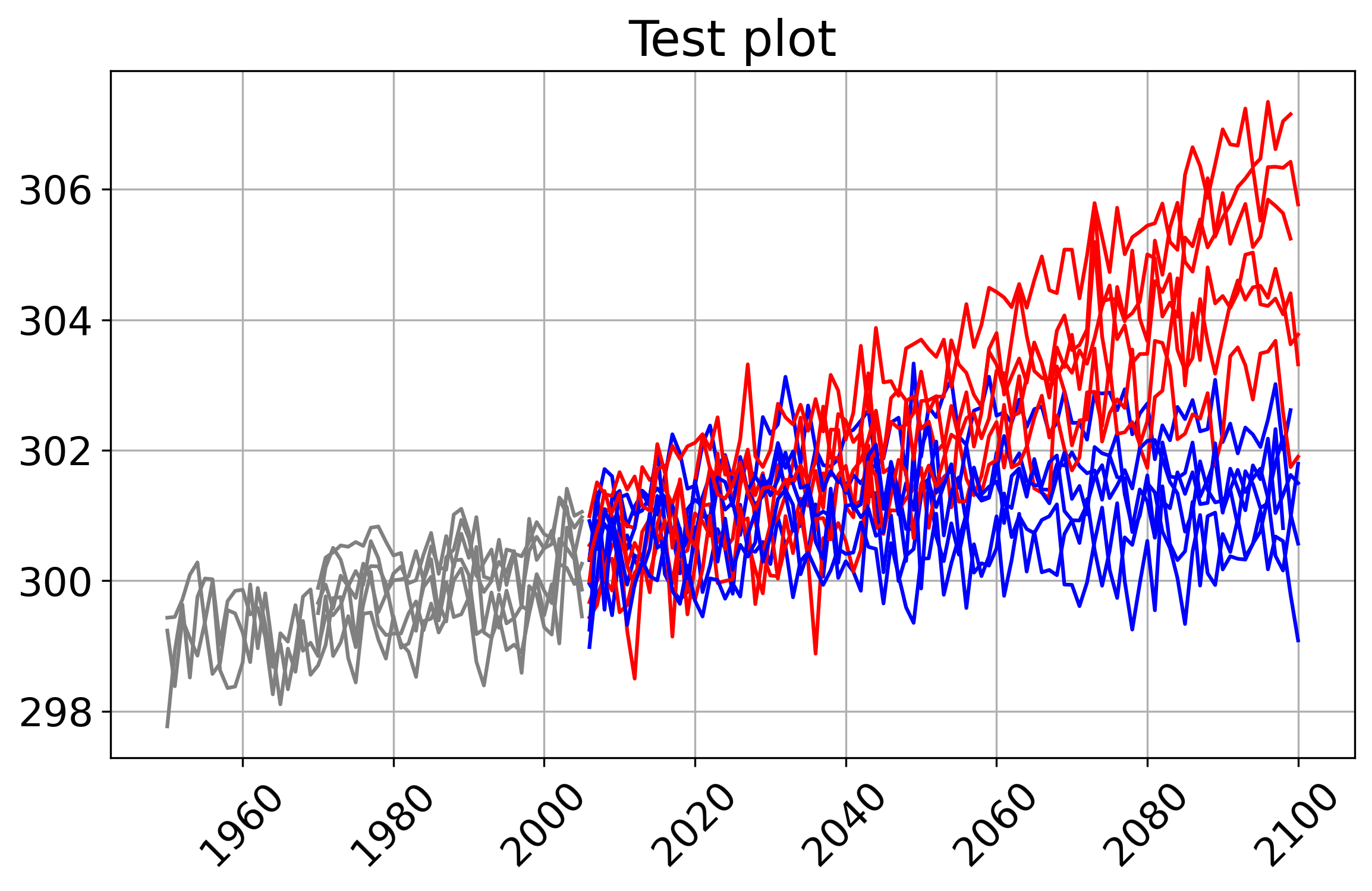
Spaghetti Plot

A simple way of visualisation of an ensemble of datasets. The plot visualises historical and rcp runs in different colors

out_plot = fp.plot_spaghetti(resource=resource, title='Test plot',
                             delta = -273.15, # to convert K to C
                             figsize='9,5',# ymin=0, ymax=14  #
                             )
len(out_plot.get())

1

# display the output graphic url:
out_plot.get(asobj=True).plotout_spaghetti
# or with:
# Image(out.get()[0], width=400)

RCP uncertainty timeseries

An ensemble of indice files will be visualised as median and the appropriate uncertainties seperatled by historical and rcp runs.

resp = fp.plot_uncertaintyrcp(resource=resource, title='Yearly mean temperature', delta = -273.15,
                            figsize='9,5', # ymin=20, ymax=100  #
                           )

# onother way to display the output graphic.

# download the file
out_file = '/tmp/ts_uncertainty_tg-yr.png'
request.urlretrieve(resp.get()[0], out_file)

# display the graphic:
Image(out_file, width=400)

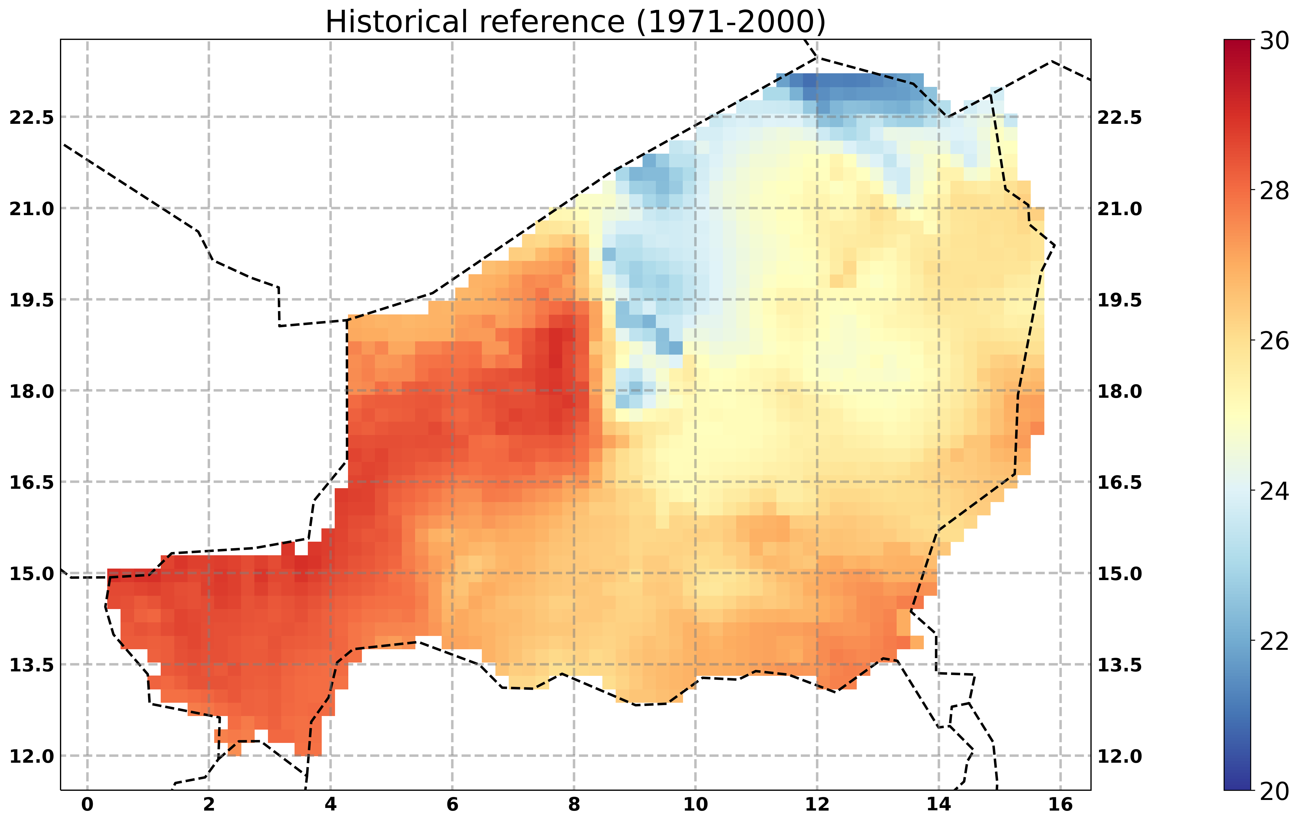
Plot a map

Spatial visualisation of data as a mean over the time.

# select only the historical runs of the indices ensemble
hist = [f for f in resource if 'historical' in f]

# process the data of the years 1971-2000
out = fp.plot_map_timemean(resource=hist, title='Historical reference (1971-2000)',
                            delta = -273.15,
                             datestart='1971-01-01', dateend='2000-12-31',  # subset a time range
                             vmin=20,  vmax=30,
#                              cmap=''
                           ) #

# display the output graphic
Image(out.get()[0], width=600)

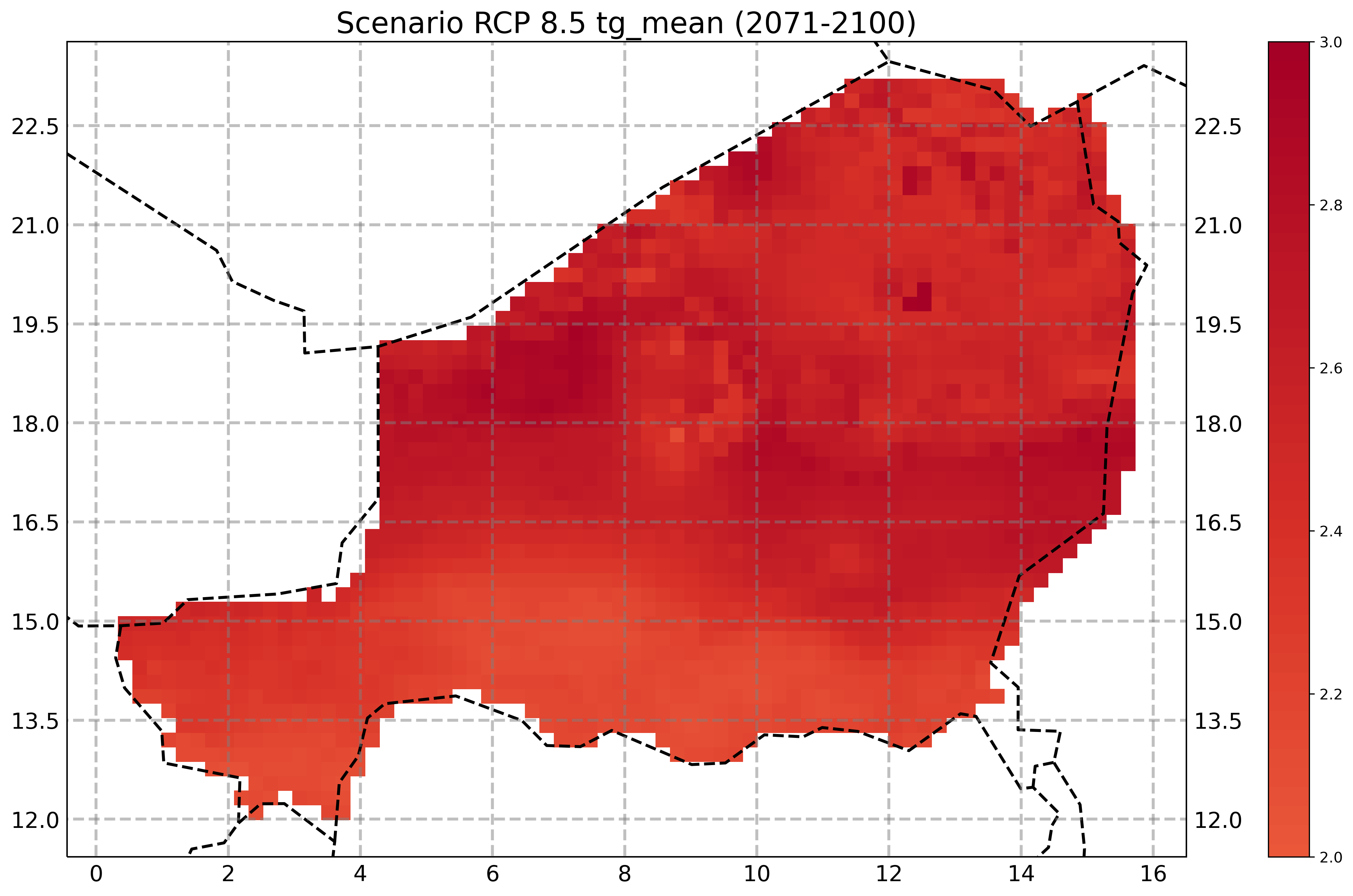
plot a climate change signal

calculation of the differnence in a climate signal between a future projection to a reference periode

dates = ['1971-01-01', '2000-12-31', '2036-01-01', '2065-12-31', '2071-01-01', '2100-12-31']

ref = [f for f in tasInd_NER if tas_indice in f  and 'historical' in f] # and fr in f
proj = [f for f in tasInd_NER if tas_indice in f and 'rcp85' in f]

ref.sort()
proj.sort()

resp = fp_i.climatechange_signal(resource_ref=ref,
                                resource_proj=proj,
#                                 variable='tg-mean',
                                title='Scenario {} {} ({})'.format('RCP 8.5', tas_indice, '2071-2100'),
                                datestart_ref=dates[0],
                                dateend_ref=dates[1],
                                datestart_proj=dates[2],
                                dateend_proj=dates[3],
#                                 vmin=0 , vmax=7,
#                                 cmap='BrBG'
                               )

# using fp_i you need to wait until the processing is complete!

timeout = time.time() + 60*1   # 1 minute from now

while resp.getStatus() != 'ProcessSucceeded':
    time.sleep(1)
    if time.time() > timeout:  # to avoid endless waiting if the process failed
        break

Image(resp.get()[2], width=600)