Process Descriptions
Following is a detailed description of processes in Flyingpigeon. As Flyingpigeon is currently dedicated to be the Testbed for Process development, existing processes (like published for flyingpigeon_version_v1.0 ) might migrate to other birds (WPS services in birdhouse) in upcoming version.
Migrated Processes:
Here comes a list of Processes already developed but currently not available in flyingpigeon. In case the processes were migrated you can see the WPS where you can find them:
Process group |
migrated to: |
brief description |
|---|---|---|
Analogs of atmospheric flow |
BLACKSWAN |
Extreme Weather Analytics |
Weather Regimes |
BLACKSWAN |
Extreme Weather Analytics |
Climate Indices |
FINCH |
Climate Monitoring |
Species Distribution Models |
Disabled |
Climate Impact |
Segetal Flora |
Disabled |
Climate Impact |
Subset Processes
Generates a polygon subset of input netCDF files. Based on an ocgis call, several pre-defined polygons (e.g. world countries) can be used to generate an appropriate subset of input netCDF files. Spatial subsetting are methods of deriving a new set of data from another set of data using interpolation techniques to generate different spatial or temporal resolutions.
The User can make the principal decisions to define the area or areas to be subsetted and in case of multiple areas wether they should stay in separate files or be merged to an unit.
Point-inspection can be seen as a special form of subsetting. On defined coordinates a 1D time-series will be generated for each coordinate point.
Note
See the Subset Processes API for detailed options and data-IO.
In case of polygon subsetting used to subset the shape of e.g. countries or continents, flyingpigeon contains prepared shapefiles. To increase the performance the shapefiles had been optimized with the following steps:
Data Visualization:
They are various ways of data visualization. In flyingpigeon are realized the basic ones of creating an ordinary graphic file. It helps to have a quick understanding of your data.
Time series visualization of netCDF files. Creates a spaghetti plot and an uncertainty plot.
Plots are generated based on matplotlib. Appropriate functions are located in eggshell.
Note
See the Plot Timeseries API for detailed options and data-IO.
Spatial Analogues
Spatial analogues are maps showing which areas have a present-day climate that is analogous to the future climate of a given place. This type of map can be useful for climate adaptation to see how well regions are coping today under specific climate conditions. For example, officials from a city located in a temperate region that may be expecting more heatwaves in the future can learn from the experience of another city where heatwaves are a common occurrence, leading to more proactive intervention plans to better deal with new climate conditions.
Spatial analogues are estimated by comparing the distribution of climate indices computed at the target location over the future period with the distribution of the same climate indices computed over a reference period for multiple candidate regions. A number of methodological choices thus enter the computation:
Climate indices of interest,
Metrics measuring the difference between both distributions,
Reference data from which to compute the base indices,
A future climate scenario to compute the target indices.
The climate indices chosen to compute the spatial analogues are usually annual values of indices relevant to the intended audience of these maps. For example, in the case of the wine grape industry, the climate indices examined could include the length of the frost-free season, growing degree-days, annual winter minimum temperature andand annual number of very cold days [Roy2017].
The flyingpigeon.processes.SpatialAnalogProcess offers six
distance metrics: standard euclidean distance, nearest neighbor,
Zech-Aslan energy distance, Kolmogorov-Smirnov statistic,Friedman-Rafsky runs
statistics and the Kullback-Leibler divergence. A description and reference for
each distance metric is given in flyingpigeon.dissimilarity and based
on [Grenier2013].
The reference data set should cover the target site in order to perform validation tests, and a large area around it. Global or continental scale datasets are generally used, but the spatial resolution should be high enough for users to be able to recognize climate features they are familiar with.
Different future climate scenarios from climate models can be used to compute the target distribution over the future period. Usually the raw model outputs are bias-corrected with the observation dataset. This is done to avoid discrepancies that would be introduced by systematic model errors. One way to validate the results is to compute the spatial analog using the simulation over the historical period. The best analog region should thus cover the target site.
The WPS process automatically extracts the target series from a netCDF file using geographical coordinates and the names of the climate indices (the name of the climate indices should be the same for both netCDF files). It also allows users to specify the period over which the distributions should be compared, for both the target and candidate datasets.
An accompanying process flyingpigeon.processes.PlotSpatialAnalogProcess
can then be called to create a graphic displaying the dissimilarity value.
An example of such graphic is shown below, with the target location indicated
by a white marker.
Note
See the Spatial Analogs API for a description of both processes.
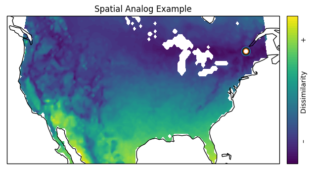
A map of the dissimilarity metric computed from mean annual precipitation and temperature values in Montreal over the period 1970-1990.
References
- Roy2017
Roy, P., Grenier, P., Barriault, E. et al. Climatic Change (2017) 143: 43. doi:10.1007/s10584-017-1960-x
- Grenier2013
Grenier, P., A.-C. Parent, D. Huard, F. Anctil, and D. Chaumont, 2013: An assessment of six dissimilarity metrics for climate analogs. J. Appl. Meteor. Climatol., 52, 733–752, doi:10.1175/JAMC-D-12-0170.1